
⚡️Hacking the Power System. An End-to-End Machine Learning Project. Part 3: Machine Learning Modeling💡

Photo: energepic.com, https://www.pexels.com/@energepic-com-27411
If you want to see this ML Model deployed, please go to:
- StreamLit App: https://jasantosm-emisiones-co2-sistema-electrico-streamlit-app-os0itf.streamlitapp.com
- REST API: https://emisionesco2api-scabs6wl2q-ue.a.run.app/docs
With this article series, I'll show you how I developed a truly End-to-End DataScience and Machine Learning Project.
Consequently, the project’s main goal is to analyze and model the technical, economic, and environmental behavior of the Colombian electric power system in an end-to-end project.
In this third part, I will show you how I designed several Machine Learning experiments to find the best algorithm to model these time series data.
However, here I will only explain what steps I executed, with some code of course, but not show much of it, for code, just go to the repository:
 jasantosm
If you are looking for the first or second part:
 Julian Santos
 Julian Santos
All images were created by the author unless explicitly stated otherwise.
Machine Learning Goals
- Understand the general behavior of polluting gas emissions from the national interconnected system.
- Determine the correlation of the amount of emissions to other variables of the electricity generation system.
- Understand the influence of climatic phenomena on SIN emissions.
- Find the influence of fuel consumption on the price of electricity.
- Create a Machine Learning Model to predict the CO2 Equivalent emissiones of the electrical system.
Tools
The following Libraries were used in this project:
- pandas
- matplotlib
- seaborn
- scikit-learn
General Defintions
- National Interconnected System (SIN): It is in fact the colombian power system that is interconected all over the country, serving most of the country.
- XM S.A. E.S.P.: It's a company part of the ISA group that is in charge of the administration of the electricity market in Colombia, it also operates the National Interconnected System (SIN), integrating its resources of generation, interconnection and transmission of electrical energy.
- Polluting Emissions: It is the discharge of gaseous fluids, pure or with suspended substances that are residues of human activity or nature and that cause adverse effects on the earth's atmosphere, such as the greenhouse effect or acid rain.
- 𝐶𝑂2: Carbon dioxide, polluting gas of the atmosphere which produces greenhouse effect.
- 𝐶𝐻4: Methane, a polluting gas in the atmosphere, which produces a greenhouse effect with a global warming potential 21 times greater than 𝐶𝑂2.
- 𝑁2𝑂: Nitrous Oxide, a polluting gas in the atmosphere, which produces a greenhouse effect with a global warming potential 310 times greater than 𝐶𝑂2.
- 𝐶𝑂2𝑒𝑞: Emissions of a gas equivalent to 𝐶𝑂2, it is calculated with the following formula 𝑇𝑜𝑛𝐶𝑂2𝑒𝑞=(𝑇𝑜𝑛𝐺𝑎𝑠)(𝐺𝑊𝑃), where GWP is the global warming potential.
Electrical System Variables
- Generation: It is the amount of electrical energy generated by the SIN.
- Demand: It is the amount of electrical energy demanded by the consumers of the SIN.
- Actual Availability: It is the installed capacity, assets ready to generate, that are capable of starting to generate energy immediately.
- Energy Contributions: These are the water contributions of the rivers and rain to the SIN's reservoirs , instead of flow, they are presented in energy units, which directly says how much electricity is capable of generating that amount of water.
- Useful Volume: It is the useful volume of water that the SIN reservoirs have, that is, with the capacity to generate energy, as well as the contributions, it is measured in energy.
- Fuel Consumption: It is the amount of fossil fuel used by the SIN.
- Exchange Price: The price of the wholesale energy exchange of the SIN.
- Emissions: For each of the polluting gases, it represents the quantity in tons of that gas, which the system discharges into the atmosphere. It only includes gases generated directly by plants burning fuel to generate.
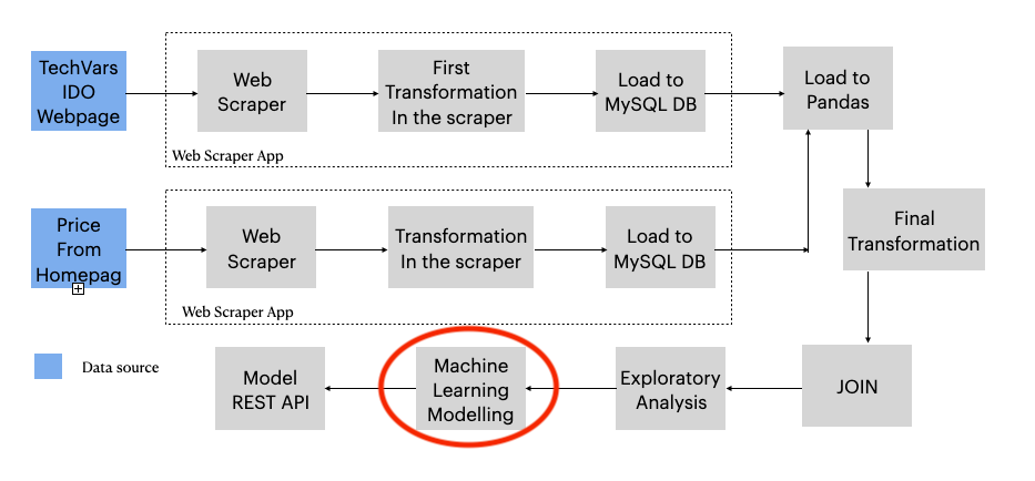
The Data
The data were extrated using the following resources:
- Web Scraper, see part 1.
- XM S.A. E.E.P. REST API
df_power_co = pd.read_csv('./data/clean_dataset/power_system.csv')Your can downlad the dataset frome here: https://github.com/jasantosm/Emisiones-CO2-Sistema-Electrico-Machine-Learning/blob/master/data/clean_dataset/power_system.csv
>>> df_power_co.info()

<class 'pandas.core.frame.DataFrame'>
RangeIndex: 2653 entries, 0 to 2652
Data columns (total 10 columns):
 #   Column                      Non-Null Count  Dtype
---  ------                      --------------  -----
 0   Unnamed: 0                  2653 non-null   int64
 1   Date                        2653 non-null   object
 2   daily_generacion            2653 non-null   float64
 3   daily_consumo_combustible   2653 non-null   float64
 4   daily_demanda               2653 non-null   float64
 5   daily_aportes_energia       2653 non-null   float64
 6   daily_volumen_util_energia  2653 non-null   float64
 7   daily_disponibilidad_real   2653 non-null   float64
 8   daily_precio_bolsa          2653 non-null   float64
 9   daily_emision_CO2_eq        2653 non-null   float64
dtypes: float64(8), int64(1), object(1)
memory usage: 207.4+ KB
Dataset time window:
>>> df_power_co['Date'].head(1)
0    2013-10-01
Name: Date, dtype: object

>>> df_power_co['Date'].tail(1)
2652    2021-01-04
Name: Date, dtype: object
The dataset time window starts on October 1, 2013 and ends on January 4, 2021
Units and conversion
The following table shows the current measurement units of the dataset and the units to which the conversion was made in order to have a more adequate management of the magnitudes.
| Variable (Feature) | Unit | Coverted to | Meaning |
|---|---|---|---|
| daily_generacion | kWh | GWh | Generation |
| daily_emision_CO2 | Ton | Ton | CO2 Emissions |
| daily_emision_CH4 | Ton | Ton | CH4 Emissions |
| daily_emision_N2O | Ton | Ton | N2O Emissions |
| daily_consumo_combustible | MBTU | MMBTU | Fuel consumption |
| daily_demanda | kWh | GWh | Demand |
| daily_aportes_energia | kWh | GWh | Energy Contributions |
| daily_volumen_util_energia | kWh | GWh | Useful Volume |
| daily_disponibilidad_real | MW | GWh* | Actual Availability |
| daily_precio_bolsa | COP/kWh | COP/kWh | Market Price |
Real availability is given in MW of power available to generate electricity, however this unit is not compatible with the energy units that manage the other variables.
For this reason, the calculation of the average real energy availability per day is made, which consists of multiplying the unit of power by the 24 hours of the day.
Experimentation Plan
For this project I am going to evaluate the following scikit-learn models:
- Multilayer Perceptron - MLPRegressor
- Random Forests - RandomForestRegressor
- Support Vector Machines - SVR
- Random Forests with gradient boosting - XGBoost
These models were selected for their power to work nonlinear problems.
The metrics with which the models will be evaluated are:
- mean_absolute_error
- mean_square_error
- r2_score
Also, I will use the forward chaining cross validation for time series.
A look to CO2 Equivalent Variable
We want to forcast the 𝐶𝑂2𝑒𝑞, which is the sum of all the CO2 equivalent emissions of CH4 and N2O, so let's take a look of it:
>>> df_CO2_ts = df_power_co[['Date','daily_emision_CO2_eq']].set_index('Date')
>>> df_CO2_ts.describe()| daily_emision_CO2_eq | |
|---|---|
| count | 2653.000000 |
| mean | 30415.946459 |
| std | 12885.491676 |
| min | 6734.720000 |
| 25% | 20722.350000 |
| 50% | 28767.140000 |
| 75% | 37956.930000 |
| max | 71519.160000 |
>>> df_CO2_ts.plot(rot=90, figsize = (12, 5), fontsize = 13.5);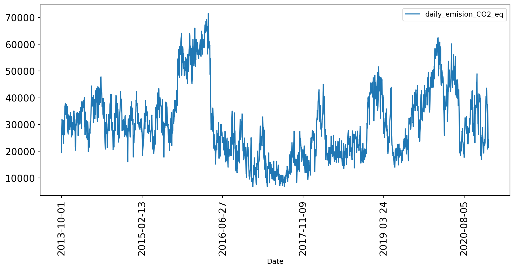
The numbers of CO2 Equivalent are to big for a Machine Learning Model, so it's a good idea to apply an standarization method to reduce their scale.
>>> from sklearn.preprocessing import StandardScaler

>>> scaler = StandardScaler()

>>> df_CO2_ts['daily_emision_CO2_eq'] = scaler.fit_transform(df_CO2_ts['daily_emision_CO2_eq'].values.reshape(-1, 1))

>>> df_CO2_ts.plot(rot=90, figsize = (12, 5), fontsize = 13.5);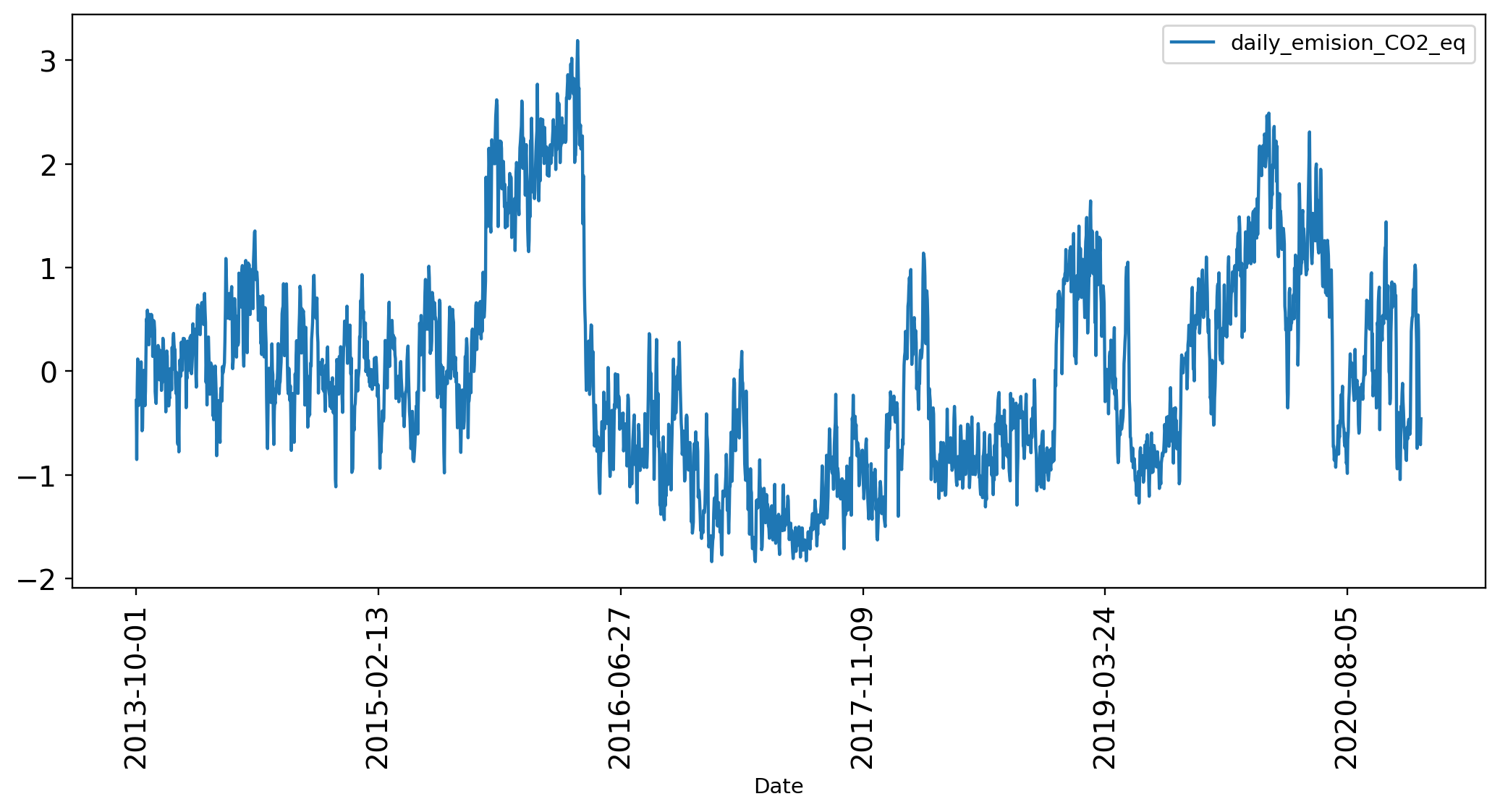
Time Series Cross Validation
A time series problem could be transform to a supervised learning problem creating a window of k backwards obserbations as predictors to estimate k1.
For the problem I will use the Forward Chaining approach:
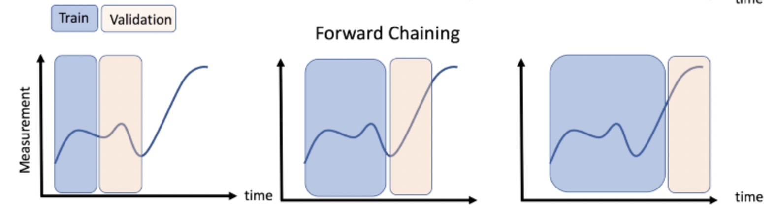
I recommend you to read the following article to have a complete explanation of a Time Series Machine Learning Regression Framework: https://towardsdatascience.com/time-series-machine-learning-regression-framework-9ea33929009a
With the following code I adapted the dataset for the ML Models.
For training data:
>>> def sliding_time(ts, window_size=1):
n = ts.shape[0] - window_size
X = np.empty((n, window_size))
y = np.empty(n)
for i in range(window_size, ts.shape[0]):
y[i - window_size] = ts[i]
X[i- window_size, 0:window_size] = np.array(ts[i - window_size:i])
return X, y
>>> data_train = df_CO2_ts['daily_emision_CO2_eq'].loc[:'2018-10-01'] #First 5 years
>>> data_test = df_CO2_ts['daily_emision_CO2_eq'].loc['2018-10-02':] #Last 2 years
>>> # Creation of the time windows for training
>>> k=20
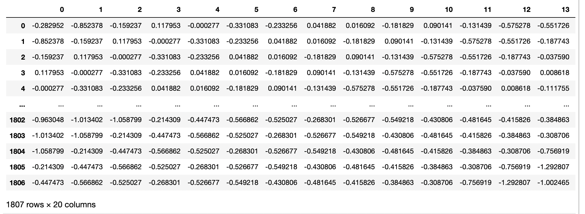
>>> X_train, y_train = sliding_time(data_train.values, window_size=k)
>>> print(f"Number of examples for training: {X_train.shape[0]} (Window size: {X_train.shape[1]})")
Number of examples for training: 1807 (Window size: 20)
>>> print(f"Number of values to predict: {y_train.shape[0]}")
Number of values to predict: 1807For validation data:
>>> X_test, y_test = sliding_time(data_test.values, window_size=k)

>>> print(f"Number of examples for training: {X_test.shape[0]} (Window size: {X_test.shape[1]})")
Number of examples for training: 806 (Window size: 20)

>>> print(f"Número de valores a predecir: {y_test.shape[0]}")
Number of values to predict: 806
The X_train dataset looks something like:
Finally, I will creat the validation partition using the Forward Chaining approach:
# Selección de los datos en series de tiempo
from sklearn.model_selection import TimeSeriesSplit

n_splits = 6

# La partición nos devuelve los indices de train y test.
tsp = TimeSeriesSplit(n_splits=n_splits)

i = 0
fig = plt.figure(figsize = (12,6), dpi = 110)
plt.set_cmap('Paired')

tsp_indexes = [(train_index, test_index) for (train_index, test_index) in tsp.split(X_train, y_train)]

for train_index, test_index in tsp_indexes:
  plt.plot(train_index,
           np.full(len(train_index), 1-i*0.001),
           lw = 8,
           ls= '-.',
           label = f'Entrenamiento (k = {i + 1})')

  plt.plot(test_index,
           np.full(len(test_index), 1-i*0.001),
           lw = 8,
           ls= '-',
           label = f'Validación (k = {i + 1})')
  i+=1
fig.get_axes()[0].get_yaxis().set_visible(False)
plt.legend(ncol=1, title = 'Índices por partición', );
plt.title('Particiones de entrenamiento y prueba')
plt.show()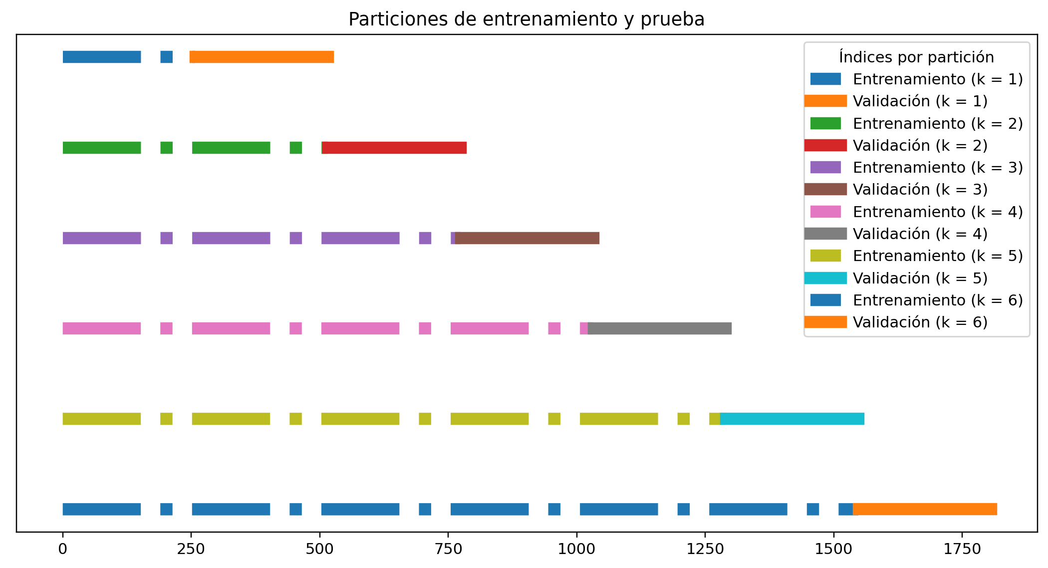
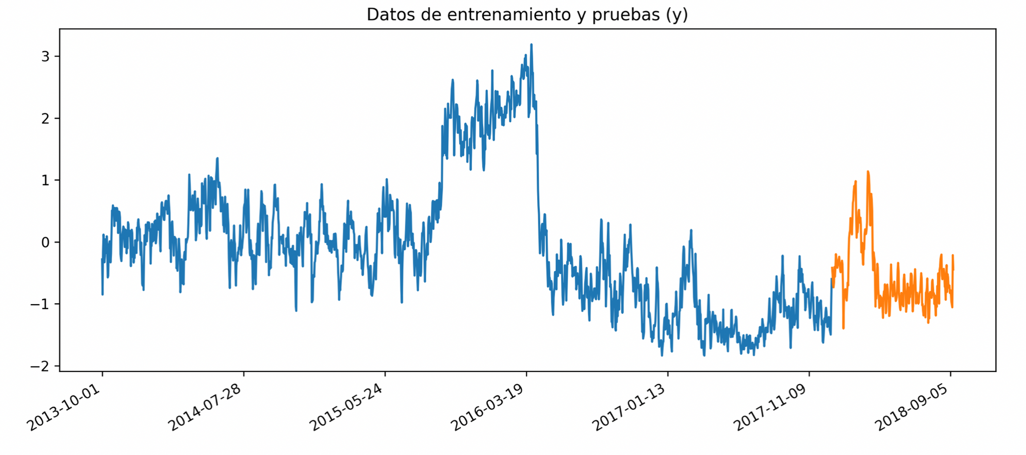
So in the next chart are represented the CO2 eq emissions time series for the K=6 dataset is, blue is training set, orange validation set:
Multiple Features
We just take a look of the variable we want to predict, the CO2 Equivalent emissions of the colombian power system. However, as you read above, the system has more variables, or features, that could help us to have a better model.
So let's take a look at them ussing the correlaction matrix plotted in a heat map:
corr_matrix = df_power_co.corr(method='spearman')
sns.heatmap(corr_matrix, vmin=-1, vmax=1);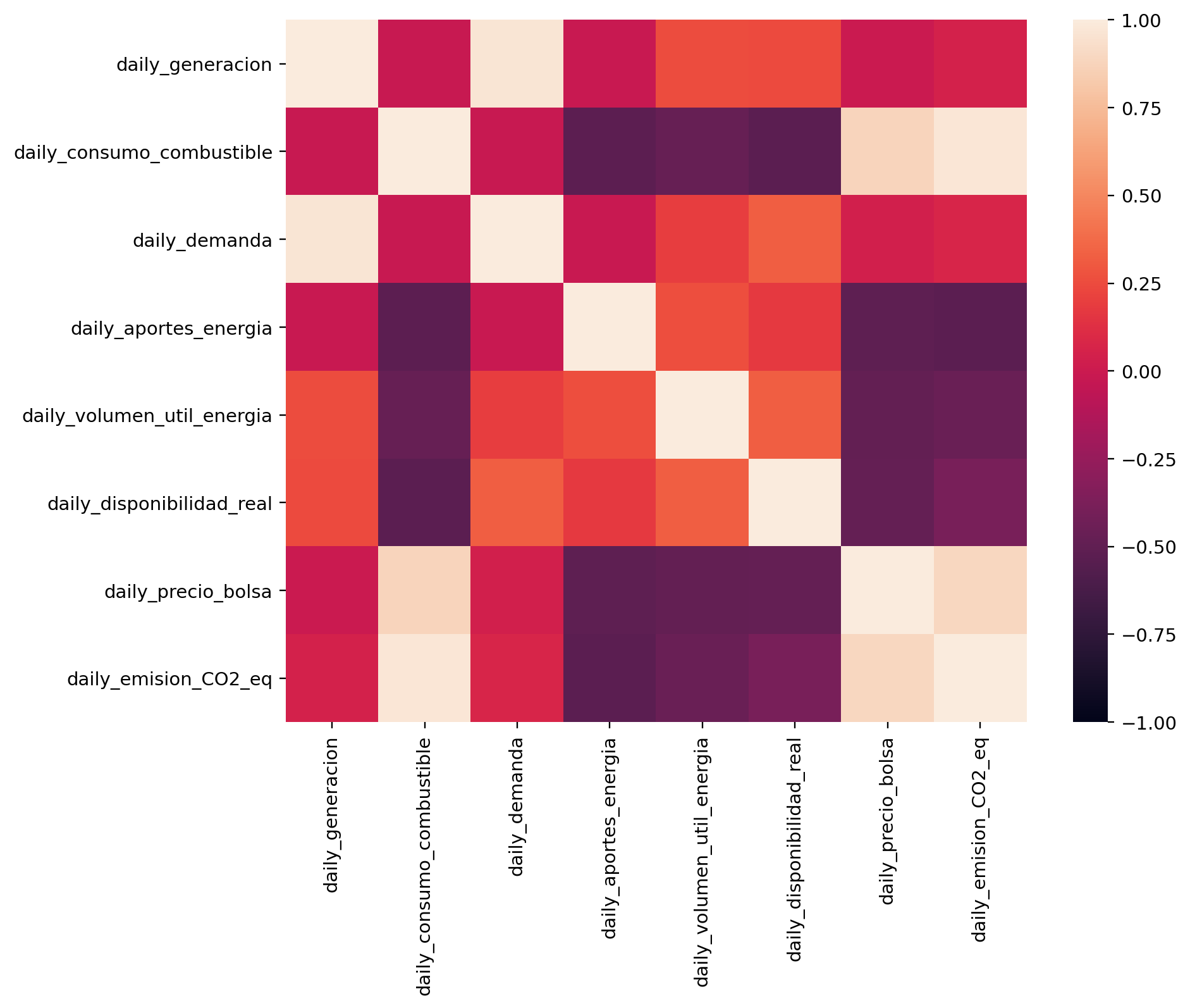
From this correlations we can conclude, that the following variables have a direct relationship with the emissions of 𝐶𝑂2𝑒𝑞:
- Fuel consumption (0.968)
- Market price (0.893)
- Demand (0.072)
- Generation (0.049)
And the following variables have an inverse relationship with emissions 𝐶𝑂2𝑒𝑞:
- Energy contributions (-0.528)
- Useful energy volume (-0.457)
- Actual availability (-0.384)
These relationships are shown below:
sns.pairplot(df_power_co,y_vars=['daily_emision_CO2_eq']);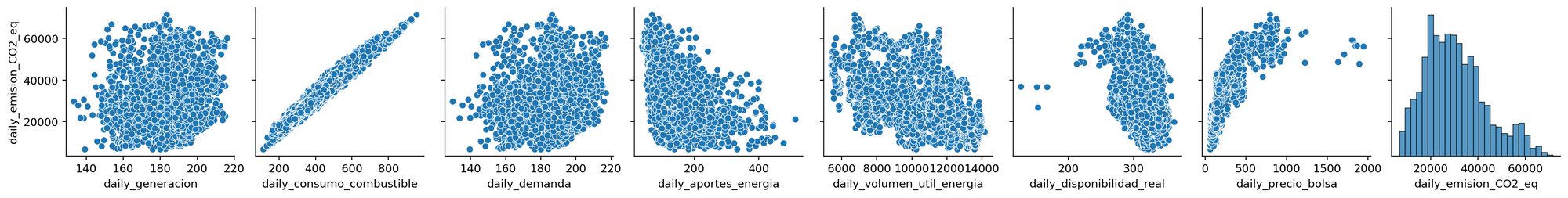
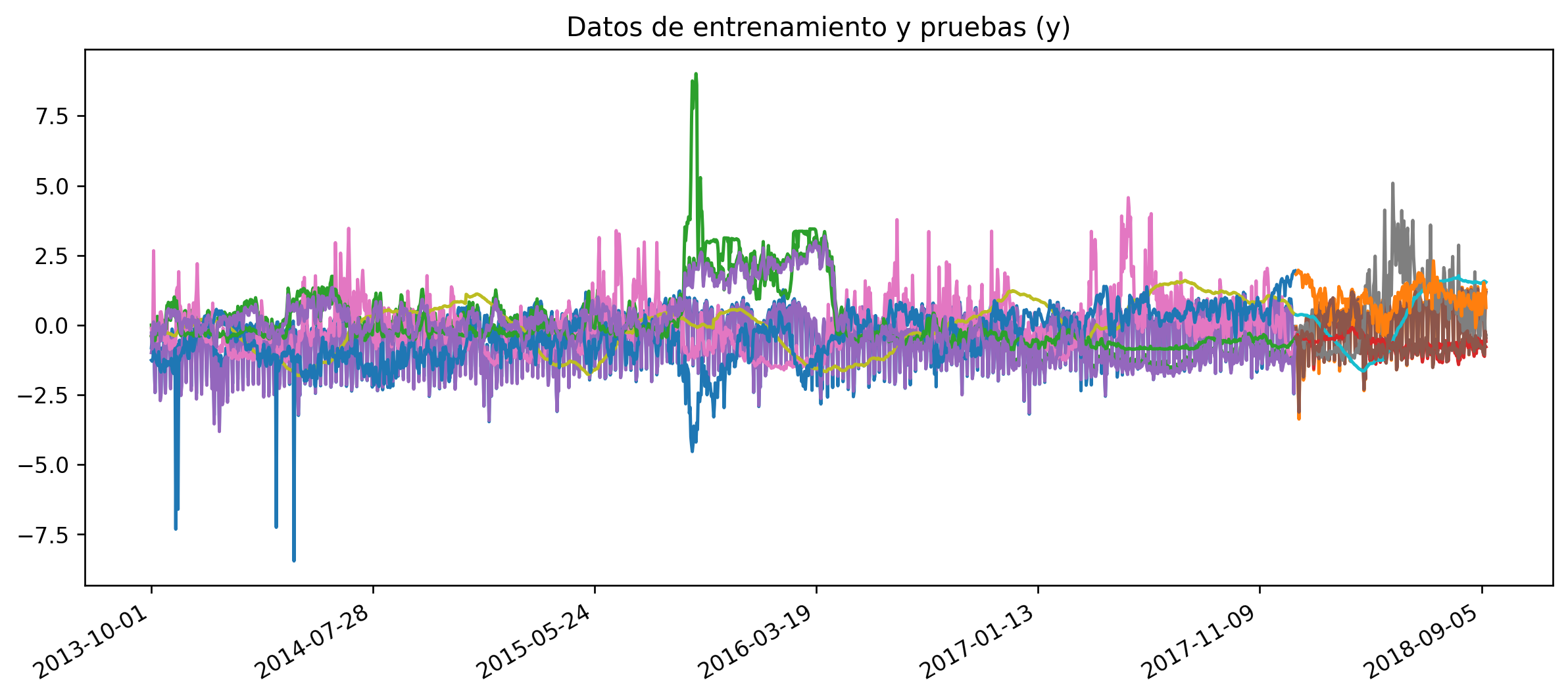
These variables most have the same processing we did for the CO2 Emissions, apply the standar scaler, vivide for train and validation using the Forward Chaining approach, and we got something like this:
Model Training and Selection
After all the data prep we finally arrive to the fun part, model training and selecction.
We will test the following algorithms:
- Multilayer Perceptron - MLPRegressor (MLP)
- Random Forests - RandomForestRegressor (RFR)
- Support Vector Machines - SVR (SVM)
- Random Forests with gradient boosting - XGBoost (XGB)
For each model we will try several hyperparameters using GridSearchCV.
The best 10 hyperparameter set of every model will be store in a pandas DataFrame, so at the end of the experimentation we will have 40 models, from that we select the best one organizing the DataFrame by mean_test_score which is the result of GridSearchCV. R2 Coefficient is used by GridSearchCV to calculate the scores.
In order to not fill the article of repetitive code I will show you how I implemented this estrategy with one model, Support Vector Machines - SVR, with the other ones is just to do the same.
params_SVR = {'C': [1, 10, 100, 1000],
          'kernel': ['rbf','poly'],
          'gamma': [0.01,0.001, 0.0001],
          'degree': [2,3,4,5,6,8],
          'epsilon': [0.1,0.2]}

tsp = TimeSeriesSplit(n_splits = 3)

gsearch = GridSearchCV(estimator = SVR(),
                        cv = tsp,
                        param_grid = params_SVR,
                        verbose = 3)

gsearch.fit(X_train, y_train)
Fitting 3 folds for each of 288 candidates, totalling 864 fits
[CV] C=1, degree=2, epsilon=0.1, gamma=0.01, kernel=rbf ..............
[CV] C=1, degree=2, epsilon=0.1, gamma=0.01, kernel=rbf, score=-0.299, total= 0.1s
[CV] C=1, degree=2, epsilon=0.1, gamma=0.01, kernel=rbf ..............
[Parallel(n_jobs=1)]: Using backend SequentialBackend with 1 concurrent workers.
[Parallel(n_jobs=1)]: Done 1 out of 1 | elapsed: 0.1s remaining: 0.0s
[CV] C=1, degree=2, epsilon=0.1, gamma=0.01, kernel=rbf, score=-3.389, total= 0.3s
[CV] C=1, degree=2, epsilon=0.1, gamma=0.01, kernel=rbf ..............
[Parallel(n_jobs=1)]: Done 2 out of 2 | elapsed: 0.4s remaining: 0.0s
[CV] C=1, degree=2, epsilon=0.1, gamma=0.01, kernel=rbf, score=0.715, total= 0.5s
[CV] C=1, degree=2, epsilon=0.1, gamma=0.01, kernel=poly .............
[CV] C=1, degree=2, epsilon=0.1, gamma=0.01, kernel=poly, score=0.658, total= 0.1s
[CV] C=1, degree=2, epsilon=0.1, gamma=0.01, kernel=poly .............
[CV] C=1, degree=2, epsilon=0.1, gamma=0.01, kernel=poly, score=-6.252, total= 0.3s
[CV] C=1, degree=2, epsilon=0.1, gamma=0.01, kernel=poly .............
[CV] C=1, degree=2, epsilon=0.1, gamma=0.01, kernel=poly, score=-0.859, total= 0.7sOrganizing the best models:
best_SVM_models = pd.DataFrame(gsearch.cv_results_).nlargest(10, 'mean_test_score')
best_SVM_models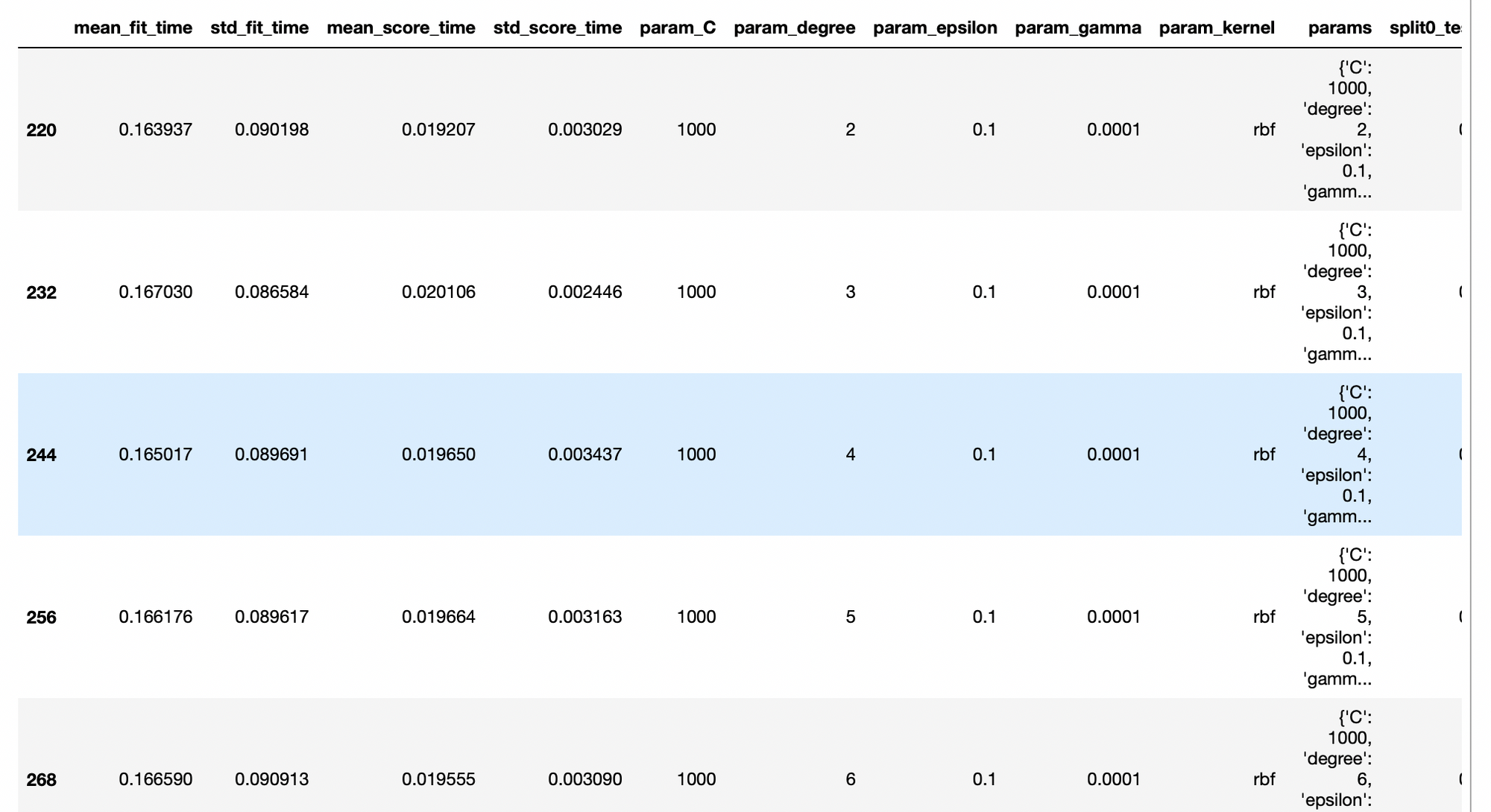
The overall metrics suggest that the best model is a Support Vector Machine regressor with the parameters:
{'C': 1000, 'degree': 2, 'epsilon': 0.1, 'gamma': 0.0001, 'kernel': 'rbf'}So we retrain the SVM algorithm with that hyperparameters:
svr_rbf = SVR(C=1000, degree= 2, epsilon= 0.1, gamma= 0.0001, kernel='rbf')
svr_rbf.fit(X_train, y_train)
y_pred = svr_rbf.predict(X_test)
x = data_test.index[k:]

fig = plt.figure(dpi = 120, figsize = (12, 5))
plt.plot(x, y_test, ls = "--", label="Valor verdadero (pruebas)")
plt.plot(x, y_pred, ls = '-', label="Valor predicho (pruebas)")
plt.title("Predicción vs valores verdaderos (pruebas) - SVR")
plt.xticks(np.arange(0, 1000, 100))
plt.legend();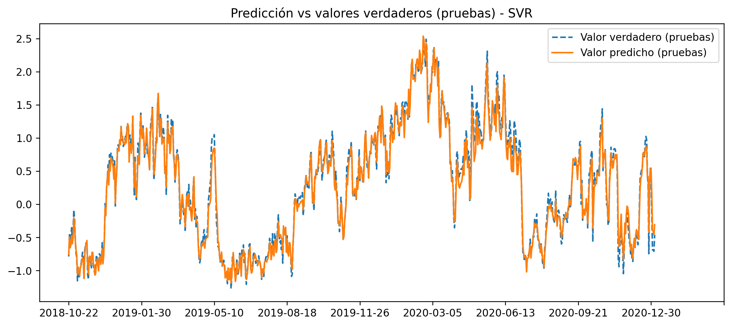
I also calculated the r2 for each model indepently, so you could see the differences:
{'y_MLP': 0.9055978712322087,
 'y_RFR': 0.8495165657123944,
 'y_SVM': 0.9855505389592659,
 'y_XGB': 0.8799233166644396}
It's clear that for this problem the best model is the Support Vector Machines.
Conclusion
With this project, and article series, I have been implementing and showing an end to end Machine Learning Engineering problem from scracth, with real data.
In this particular part 3 it was implemented a Machine Learning Experimentation plan to select the best fit for the data and be able to predict the emissions of green house gases of the Colombian power system.