Apr 17, 2021 11 min read Data Science

⚡️Hacking the Power System. An End-to-End Machine Learning Project. Part 2: Exploratory Data Analysis💡

The picture was taken by the author in Central Hidroeléctrica del Guavio, Colombia

With this article series, I'll show you how I developed a truly End-to-End DataScience and Machine Learning Project.

Consequently, the project’s main goal is to analyze and model the technical and economic behavior of the Colombian electric power system in an end-to-end project.

In this second part, I will show you how I developed the data wrangling and the Exploratory Data Analysis with Python.

*In red what we will cover in this article.*

However, here I will only explain what steps I executed to transform the data with some code, I will not show much of it, for that, just go to the repository: https://github.com/jasantosm/PowerCO_EDA_Analysis

Why no much code? Because I want to do the Exploratory Data Analysis deeply.

If you are looking for the first part:

In the third and fourth parts, I will explain the modeling using time series analysis and machine learning algorithms. Cooming Soon!

All images were created by the author unless explicitly stated otherwise.

Data Wrangling

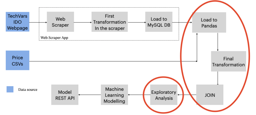
As I showed in the first part, the data collected with the scraper is continuously stored in a MySQL DataBase.

Because of that, we take the data from 2013.10.01 to 2021.01.04 to do the whole process (EDA, time series analysis, and ML) in a batch way.

Therefore, the data is downloaded from the database to CSV files and then loaded to Pandas.

operation_data.csv
prices.csv

Note that, this is a manual process, at the very end of the project, the idea is to create a whole MLOps pipeline to do all of this automatically.

If you want to know more about MLOps, look at this Google Article.

Scraped Data Structure

The CSV data from the scraper database has the following columns and types:

#Operation Data CSV structure and types

date                                      object 
generacion_total_programada_redespacho    object 
generacion_total_programada_despacho      object 
generacion_total_real                     object 
importacion_programada_redespacho         object 
importacion__real                         object 
exportacion_programada_redespacho         object 
exportacion__real                         object 
disponibilidad_real                       object 
demanda_no_atendida                       object 
costo_marginal_promedio_redespacho        object 
aportes_hidricos                          object 
volumen_util_diario                       object 
volumen                                   object 
id                                         int6

These columns represent the operational variables of the Colombian power system each day. Below, there is the price CSV structure and types as well.

#Prices Data CSV structure and types

id                    int64 
date                 object 
precio_bolsa_tx1    float64

Unit Conversions

Before the transformation of the DataFrames, we have to make some unit clarifications and conversions.

In effect, we are dealing with a technical problem, for this reason, it’s important to have clear the variable meaning and units:

precio_bolsa_tx1: This is the market energy price in COP/kWh
generacion_total_programada_redespacho: Planned redispatch generation in GWh
generacion_total_programada_despacho: Planned generation in GWh
generacion_total_real: Actual total generation in GWh
importacion_programada_redespacho: Planned energy importation in GWh
importacion_real: Actual energy importation in GWh
exportacion_programada_redespacho: Planned energy exportation in GWh
exportacion__real: Actual energy exportation in GWh
disponibilidad_real: Actual availability MW
demanda_no_atendida: Not attended demand MWh
costo_marginal_promedio_redespacho: Cost in COP/kWh
aportes_hidricos: Water contribution to the reservoirs system in GWh
volumen_util_diario: Water useful volume in the reservoirs system units in GWh
volume: Total water volume in the reservoirs GWh

When the IDO Page does not report a value, or there is a mistake, the scraper save a “ND” in the affected value. (ND stands for no-data)

In the electric sector, it’s prevalent to use as energy unit Giga-watts-hour (GWh), instead of Jules (J).

Maybe you are wondering why to use a power unit as an energy unit. Just think that 1 Wh is the energy necessary to maintain a constant power in a motor of 1 W for one hour.

Another practical way to see it is that the generation capacity of the power plants are expressed in MW or GW, so it’s easy to compare.

Giga = 10⁹multiplier, symbol G
Mega = 10⁶ multiplier, symbol M
Watts = Power unit, symbol W = energy/time = J/s
Wh = Power unit * time unit = energy unit

The actual availability (disponibilidad_real) is originally expressed in MW, however, all the other variables are in GWh.

Therefore, if we are doing the analysis on a daily basis, we can put the time to the actual_availability units, in that case, we have the average availability during that period of time.

Average availability (GWh) = availability (MW) * 24 /1000

In the case of not attended demand (demanda_no_atendida) is just to change the multiplier from mega to giga dividing by 1000.

power_system_data['disponibilidad_real'] = power_system_data['disponibilidad_real'].apply(lambda x: x*24/1000)
 power_system_data['demanda_no_atendida'] = power_system_data['demanda_no_atendida'].apply(lambda x: x/1000)

Another important clarification regarding the units is that the volume of water is expressed in terms of the energy that is able to store, that is to say, energy in GWh instead of volume in Mm³

Data Cleaning

The DataFrames are “raw”, so it is necessary to execute the following wrangling steps over the Operation Data DataFrame:

Change ND string to zero (0)
Put the correct data type in each feature
Set ‘date’ as the index
Drop database ‘id’ field
Check for nans
Make the necessary unit conversions to have a consistent set of units
Put the data in a new DataFrame named operation_data

Over Prices DataFrame:

Set date as the index
Drop database ‘id’ field

Maybe you are wondering why I used two DataFrames, well, because the data was scraped from two different pages, so I made two independents scrapers, if one crashes, the other one could still run.

Now, it’s necessary to join both tables in one DataFrame

To do that, I used the Pandas’ merge method that works similar to SQL join statement.

power_system_data = pd.merge(prices_data, operation_data, on="date", how='outer')

Because I did an outer join, it’s possible that some values got a nan value:

>>> power_system_data.isna().sum()
>>> date                                       0 
    precio_bolsa_tx1                          36 
    generacion_total_programada_redespacho     0 
    generacion_total_programada_despacho       0 
    generacion_total_real                      0 
    importacion_programada_redespacho          0 
    importacion__real                          0 
    exportacion_programada_redespacho          0 
    exportacion__real                          0 
    disponibilidad_real                        0 
    demanda_no_atendida                        0 
    costo_marginal_promedio_redespacho         0 
    aportes_hidricos                           0 
    volumen_util_diario                        0 
    volumen                                    0 
    dtype: int64

As you see, there are 36 days without a price in the new DataFrame, that’s not much but I don’t want to lose any data, so these empty prices will be filled with the previous valid value.

power_system_data['precio_bolsa_tx1'] = power_system_data['precio_bolsa_tx1'].replace(to_replace=np.nan, method='ffill')

This kind of empty values could appear when you join two tables into one, this happens when a row exists in one table but not in the other.

As I explained before when the operation data scraper finds an error or an empty value, on a particular date, puts a “ND” value. I change that ND value for zero, so if we graph the time series, we will find corrupted values:

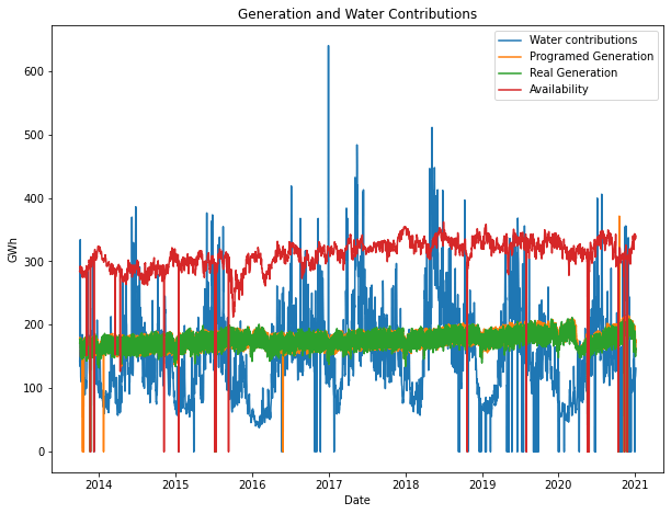
Look at that zero values, those are days where the scraper found an error or exists a price without operation data, on a particular day.

If we don’t heal that values somehow, our models will be biased.

After applying the same technique used for prices to each feature, the time series look like this:

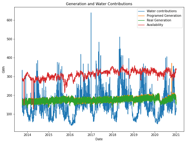
Looks better, right?

Definitely, replacing the zeros with the last valid value makes sense because it’s impossible to have those variables in zero, it has no physical or realistic meaning.

Well, now we have a beautiful set of time series to analyze 😊

General Analysis

As you probably know, if that’s possible, looking at the data graphically is the easiest way to extract insights.

So let’s take a look:

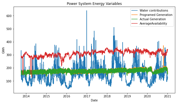
It’s gratifying to see the insights that you can discover by just plotting the time series!

Therefore, here I present the general insights I found:

It’s evident that in the fourth quarter of 2015 and the first quarter of 2016, there was a big anomaly, which we are going to analyze deeply below.
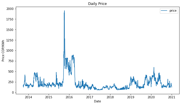
The price seems to have a stationarity time-series behavior over the time interval analyzed, which is obviously affected by other variables. We will check that in the third part.
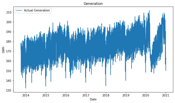
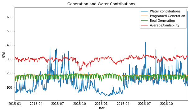
The actual generation shows a slightly positive trend over all the time interval and has two points where the trend inverts locally, at the 2015-2016 year change and at the beginning of 2020.
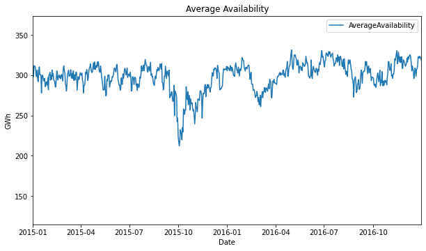
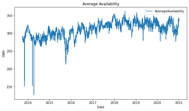
Average availability shows a slightly positive trend from 2013 to 2018 and has a very notorious dropdown at the 2014-2015 year change, and at the end of 2015. It also inverts the trend to slightly negative from 2018 to the middle of 2020.
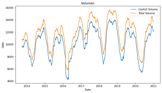
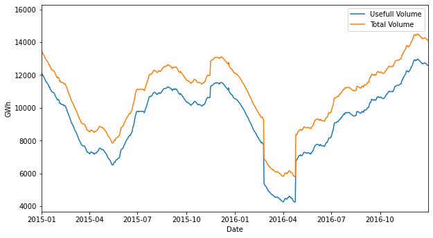
Water contributions, total and useful water volume show a clear seasonal behavior, look that is clear that the minimum is located in the first half of 2016.
There is a constant gap between total volume and useful volume.

Analysis of end-2013 to mid-2015 Period

In this period of time, there were 3 hard average-availability downs, which causes the price rise in that time.

Why the availability could make the price rise? Because there are less power plants producing the electricity enough for the system, so less supply, same demand, price goes up.

Additionally, if the less availability of the system is produced because a hydraulic power plant went out, the thermal power plants must start generation at a very higher cost.

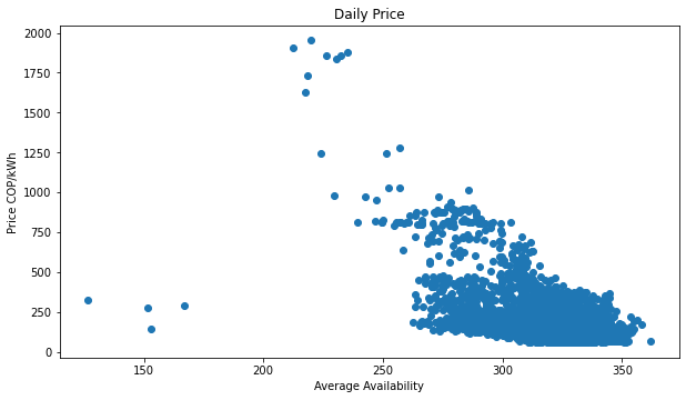
The plot shows the inverse relation of these two variables. Low availability then high price.

The power grid is a very complex system, where several entities are acting over it. If a single plant goes out can cause a hard failed of the system, because of that the price is highly correlated with the availability.

Analysis of 2015 – 2016 Period

This is the most interesting period, from October 2015 to April 2016 the variables have very different behavior.

Let’s take a closer look:

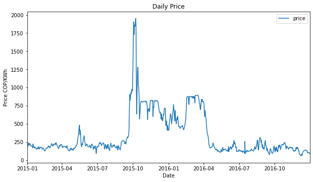
Within this interval we can find several maximums or minimums over all the analyzed time period 2013.10.01 to 2021.01.04:

The highest price 1952.18 COP/kWh, mean 225.03 COP/kWh
The lowest water contributions 37.96 GWh, mean 151 GWh
The lowest useful volume in the reservoirs 4238.35 GWh
The lowest total volume in the reservoirs 5794.62 GWh
The lowest average availability 212.4 GWh (For this analysis we consider as outliers the minimums presented in 2013 and 2014)

These numbers are so different compared to the other years, however there is a reason.

So it’s fantastic to realize that exists a very special reason for that behavior: The oceanic and climatic phenomenon called El Niño.

El Niño Event

El Niño is an oceanic and climatic phenomenon that is produced by the pacific ocean temperature increase.

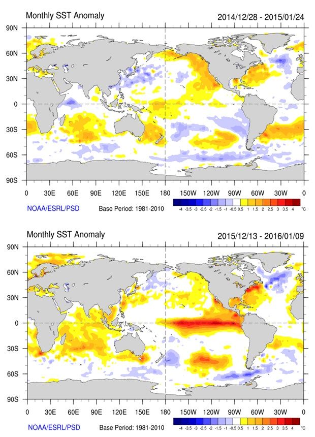
*Source: XM, http://informesanuales.xm.com.co/2015/SitePages/operacion/2-1-Condiciones-climaticas.aspx*

It produces several climatic effects all over the globe, in fact, in Colombia these effects are drought and high ambient temperatures.

In addition, the El Niño 2015/16 event was one of the strongest ever recorded, affecting Colombia in a significant way due to the very hard drought we had those days.

Regarding the temperature, the country had had the highest levels ever recorded, this caused the increase of power consumption because of the air conditioning equipment usage.

Power System Main Effects

The price was highly affected, during this period, it had the highest values, with lots of difference. During the 7 years analyzed the price mean is 225.03 COP/kWh, and in the period between August-2015 and May-2016 was 570.2 COP/kWh, which is 153.4% more expensive!

There are several reasons that explain this behavior:

At the beginning of October, the El Niño event was officially started, which means the government announced it officially, this created speculation in the market.
In order to save water for the driest months, several hydraulic power plants stopped or slowed their operation, so the natural gas and coal fired power plants started their operation to their maximum capacity, which caused the increment of the natural gas prices due to its shortage.
Also, the water-saving strategy caused the average availability to drop.

If we look at the plots, we can see that in the first months of the event, from October to December, the useful volume increased, while the water contributions decreased, that’s not logic, and it’s explained by the water-saving strategy.

Even if the energy price was high, the system demonstrated that is capable to support this kind of event, due to its capacity of balancing water-thermal generation, and also the correct saving energy strategy executed by the power grid operator. All this without the need for rationing.

Analysis of 2018 to mid 2020 Period

In December of 2018, the power grid was supposed to have 2.400 MW added to the system due to the hidroituango power plant opening. This new plant would allow the system to maintain an average availability with a slightly positive trend, however, that didn’t happen.

In May of that year, Empresas Publicas de Medellin (EPM) decided to flood the generator house of the project due to the plugging of the main water-flow tunnels, which collapsed because of the sudden increase of water flow produced by an engineering mistake.

That was a huge engineering mistake, the generators already installed were damaged without repair possibility.

That’s the reason why in this period the average availability had a slightly negative trend.

Analysis of 2020 Period

Everybody knows that 2020 has been a tough year, the coronavirus pandemic has impacted the world without precedent.

In late March, Colombia started a very hard quarantine regime that lasted more than 6 months.

April was the hardest month, where lots of companies stopped their operations.

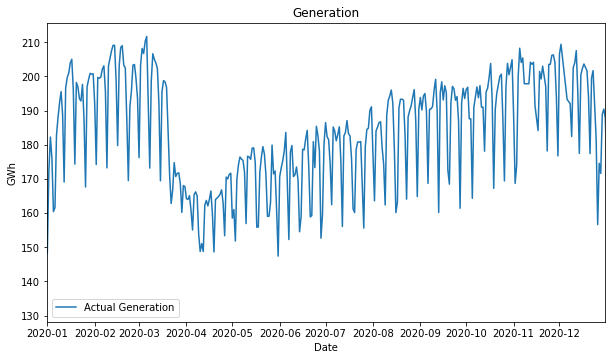
This economic stop is clearly represented in the energy generated this month. This behavior shows us that the industrial sector is a big electricity consumer, even with all the Colombians at home, these houses full of people all day long did not consume as the industry does.

Conclusions

It’s amazing what you could find in the data!

With the power grid data, we could find and analyze: operational behaviors, price changes, consequences of engineering mistakes, and even climatic events.

In later posts, I will model this data to forecast prices and electric generation.

Thanks for reading me.